Neural networks learn boundary layer meteorology

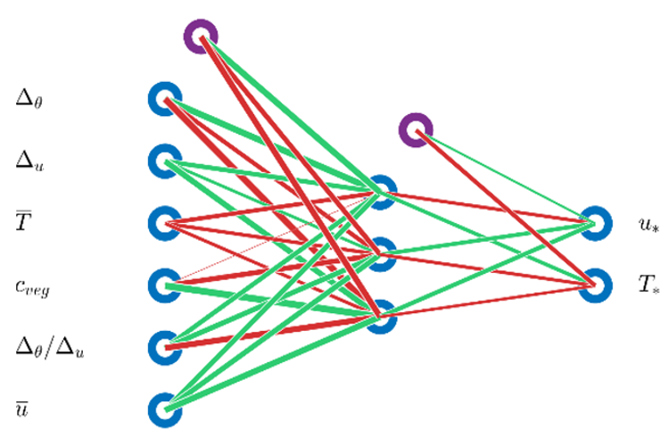
Fig. 1: The 6-3-2 neural net with six input nodes, one hidden layer and two output nodes.

The turbulent fluxes of momentum, heat, water vapour and trace gases are the link between the atmosphere and the Earth’s surface. Faithful modeling of these fluxes is therefore essential for a proper functioning of climate resp. Earth system models (and also for weather forecast models, of course). In these models, the fluxes respective covariances are parameterised using a velocity scale u* and a (potential) temperature T* scale.  u* and T* depend on near surface wind and temperature, their gradients, surface roughness and atmospheric stability. In the framework of the almost exclusively used Monin-Obukhov similarity theory, u* and T* are obtained from so-called universal stability functions which depend on a single stability parameter. These stability functions were determined empirically by different authors from regressions on observations using a small number of field experiments. Due to the limited number of and scatter within the data as well as possibly violations of the assumptions of Monin-Obukhov theory, the functions vary considerably among authors, and are especially in the very stable and the very unstable regimes not very reliable. Furthermore, the underlying non-linear equations must be solved iteratively at each time step of a model run, which can be computationally expensive.

We have used an artificial neural network (more precisely, a multilayer perceptron) to obtain the scaling quantities u* and T*. To train, validate and test the neural network, a large set of worldwide observations was used, representing tall vegetation (forests) and low vegetation (grassland, agricultural terrain). A quality assessment of the data sets showed that not all of them were compatible with Monin-Obukhov similarity theory, so only a subset of the data sets could be used. Extensive sensitivity studies showed that even a relatively small 6-3-2 network with six input parameters and one hidden layer (see Figure) can yield satisfying results. In the trade-off of quality of results vs. computational efficiency, this network performed best.  An implementation of this network in a stand-alone land surface model showed that the neural network version gives results equivalent to and sometimes better than the standard implementation. After some extensions and fine tuning to improve the computational efficiency, the neural network routine will be implemented and tested in a three-dimensional regional climate model.

Reference: Leufen, L. and Schädler, G.: Calculating the turbulent fluxes in the atmospheric surface layer with neural networks. Submitted to GMD.

[Working group: Regional Climate and Water Cycle]