
Investigation of the convectively driven boundary layer in the Inn Valley during CROSSINN
A high-resolution detection of the evolution of the convectively driven boundary layer remains a key challenge within boundary-layer meteorology. Today, adequate temporal resolution of the boundary layer top measurements can be achieved using Doppler lidars, microwave radiometers, or ceilometers. In contrast, however, comparable horizontal resolution requires both numerous advanced instruments and certain assumptions regarding flow properties. When a measurement is made in horizontally heterogeneous and mountainous terrain, such as an Alpine valley, the validity of these assumptions cannot be assumed in all cases. For example, a point measurement of the boundary layer top above a valley sidewall would be insufficiently representative for the rest of the valley. Therefore, it is of great importance to obtain high quality spatial knowledge of the boundary layer top in mountainous terrain, which can be achieved using a suitable measurement strategy.
In order to improve the understanding of processes responsible for the spatial and temporal evolution of the boundary layer top in Alpine valleys, a special field campaign was conducted in the Inn Valley, Austria. The measurement phase of the CROSSINN (Cross-valley flow in the Inn Valley investigated by dual-Doppler lidar measurements) campaign took place between 1 August and 13 October 2019. Numerous data sets were obtained using an existing network of surface flux towers and remote sensing instruments. These included three energy balance and turbulence measurement systems, six Doppler lidars, one ceilometer, one Raman lidar, and one microwave radiometer, as well as soundings using radiosondes and aircraft measurements during intensive observation periods.
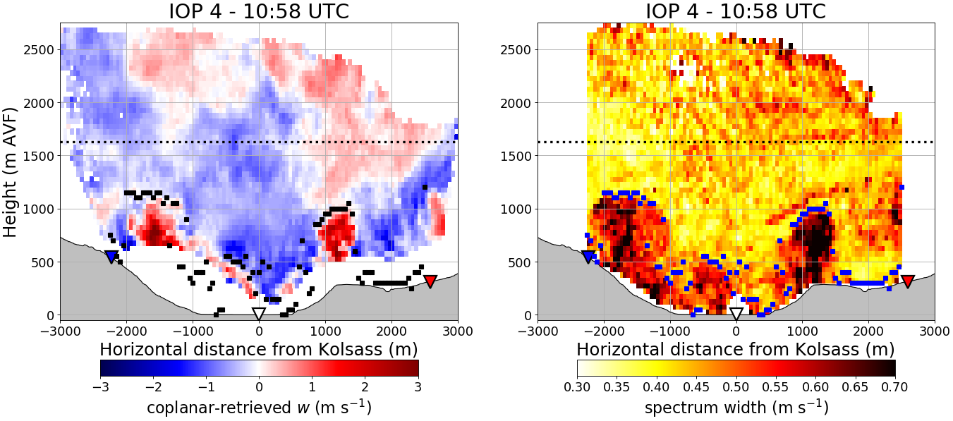
Of particular interest are three Leosphere Windcube WLS200s Doppler lidars, which are part of the KITcube observing system at IMK-TRO. These instruments detect not only the radial wind speed and backscatter, but also the spectrum width within the pulse volume, which is dominated by shear as well as buoyancy effects due to turbulence. This spectrum width property can be used to determine the boundary layer top since the free atmosphere is nearly devoid of turbulence. An example of this is shown in Fig. 1. Once a vertical cross section of spectrum width from all three Doppler lidars is compiled, the boundary layer top can be determined for each vertical profile by searching from bottom to top for an exceedance of the 0.44 m/s threshold (Fig. 1). The boundary layer top obtained in this way corresponds to the upper bound of convectively driven eddies, which are typically characterized by strong vertical updrafts.
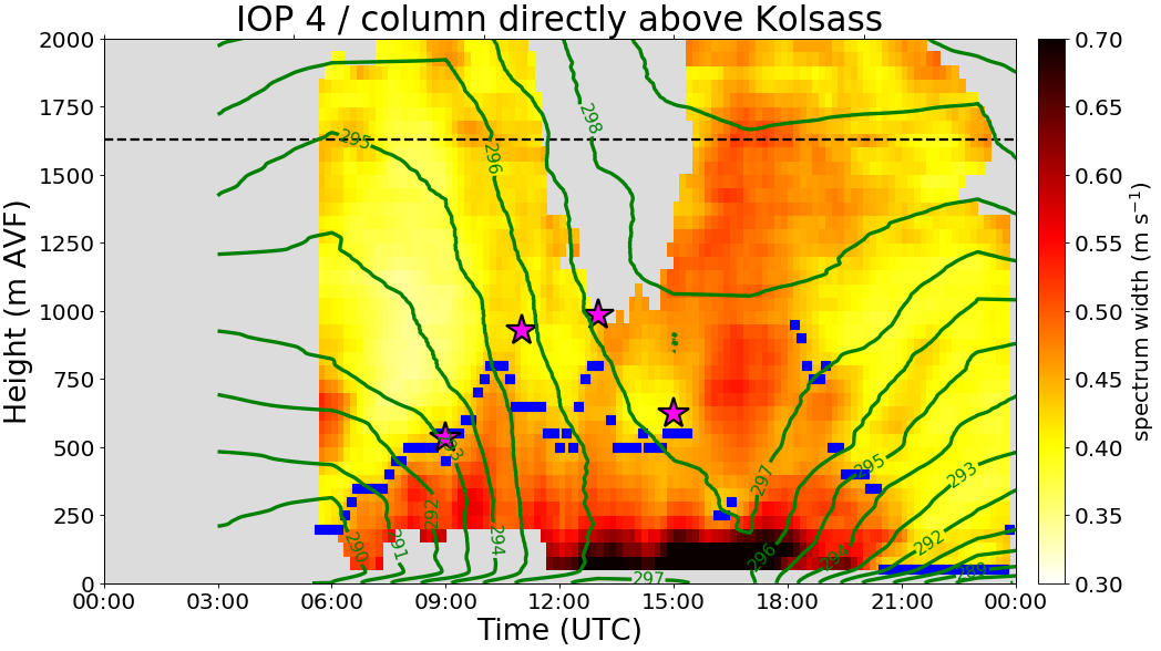
The potential of the new method can be estimated by validation using boundary layer tops obtained from the more traditional Richardson method (Fig. 2). Since the new method has been adapted for convectively driven conditions between approximately 06:00 and 14:00 UTC, its poorer performance between 15:00 and 21:00 UTC remains evident. On the one hand, this time window is characterized by a negative surface sensible heat flux that does not support convection. On the other hand, within this period a so-called cross-valley vortex was prevailing, whose strongly pronounced dynamic character covered the whole valley atmosphere, so that the necessary exceedance of the threshold was often erroneous.